Like a lot people, when the covid-19 broke out in our country and you couldn’t open the radio or the tv without hearing about it, I wondered how a pandemy spread. While the basic law derives from a simple differential equation, the reality is a bit more complicated, and the implications are much more widespread.

Simply states a pandemy is the spread of a disease from 1 person to a group of persons, rather to the whole world.  A very first question derives from this statement: if the pandemy starts with 1 person, how is this person been infected ? A lot would probably answer: from an animal.  O.K, but within the population of (all) animals, how was the first of them infected ? At the end of the chain you have the mutation of a virus that already have existed … the evolution.

Outside the possible confessional or philosophical discussions, the fact that a pandemy starts (and ends) with 1 person, imposes that the type of functions being a solution of the underlying equation have a limited domain, i.o.w. they don’t start from -∞ to extend till +∞.  Further, the continuous class of functions is not really appropriate, since there exists no decimal person, the discrete class of functions is the only one that is adapted.  Unfortunately, discrete math are much more complicated and can’t lead, as far as I know, to an algebraic (analytical discrete) solution for the type of equation we are dealing with.  Numerical solving exists, luckily.

So I will limit the following to the continuous analytical description of the phenomenon, which is sufficient to understand the basis and then afterwards extrapolate the results to a wide range of domains among which the stock exchange storms and the fashion successes.

The basic equation describing the spread of something, like an infection, within a (sane) population, relies on the relation between the evolution of the amount of newly infected (within a time interval), the amount (rather the fraction or relative amount) of people (already) infected at that moment, the amount (relative) of people not yet infected at that moment and a (global) transmission coefficient.

If we note ‘c’ the function describing the amount of infected people, ‘s’ the amount sane (not yet infected) people, at a defined time ‘t’, with ‘k’ being the transmission coefficient and ‘n’ the total amount of people in the population, we have (with dc/dt being the differential of c along t):

(dc/dt) = k . c . s, where s = n – c, thus (dc/dt) = k . c . (n – c);

in discrete form we would have: c_i+1 – c_i = k . c_i . (n – c_i), for which I haven’t found an algebraic solution (giving an expression for c_i+1 in function of c₀ and eventually some following ones).

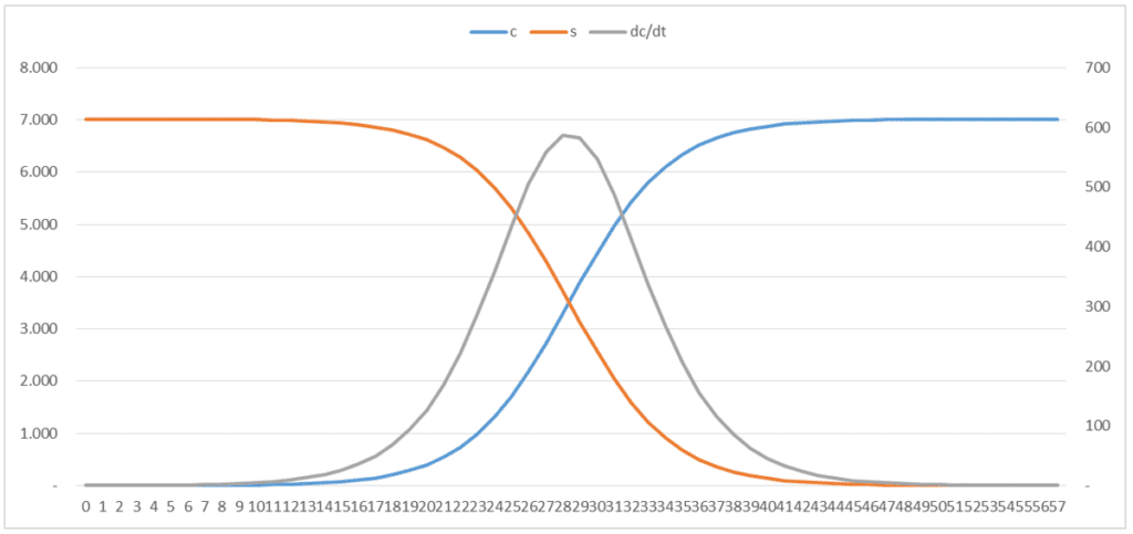
Thus ‘c’ is the amount of infected people, within a total population of ‘n’ people.  The curve figuring ‘c’ in function of the time is an S curve, starting with a value of 1 when t = 0 and ending at the time ‘t’ where c = n.  While dc/dt in function of the time is a bell curve, at first sight similar to a Gaussian one, but in reality (and analytically) totally different from this.  The values of ‘c’, ‘s’ and ‘dc/dt’ (thus the vertical axis) depend of course on the values of ‘k’ and ‘n’.

Since ‘c’ is the integral (thus the sum along the time) of ‘dc/dt’, the highest value reached by ‘c’ (and ‘s’) is much higher than the maximum of ‘dc/dt’, requiring different vertical axis for ‘c’ (or ‘s’) and ‘dc/dt’.

The analytical expression of ‘c’ (flows out solving the differential equation and applying the initial and asymptotic conditions), is: c = n / { 1 + (n-1) e^-k.n.t }, satisfying to: c = 1 when t = 0 and c = n when tends to +∞.  Of course the fact that c tends to n only when the time tends the infinite, seems annoying, but in reality infecting 100% of a population is never possible.

We see (rather can calculate) that the dc/dt curves reaches a maximum when c = n/2 (this is rather very intuitive), situation which occurs when t = [1/(k . n)] . ln (n-1), in which ‘ln’ is the Neperian logarithm.

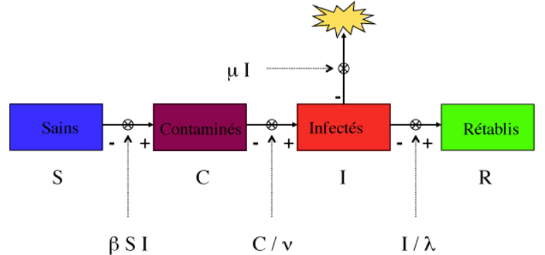
Now the real complete model for a pandemy is much more elaborate than the basic one presented above, it takes into account the difference between the contaminated people (who are not, or not yet, ill), the infected people (who are ill), the cured and the one who dies.  Below a copy of the image presented in the article published on https://interstices.info/modeliser-la-propagation-dune-epidemie/.

The solution of the underlying (differential equations) system requires numerical calculation, that are achieved in real time behind, on the above mentioned url, after you have chosen the values for the parameters.  Interesting, easy and nice to test and observe the effect of the parameters.

Roughly the basic equation for ‘dc/dt’ is identical to the one describing the transition from the stage ‘Sains’ to the stage ‘Contaminés’, in the full model above.  The other transitions are rather driven by (for each stage transition): a fraction of the population in one stage goes to the adjacent one, within each time interval.

Now, of course the models presented assume a constant value for ‘k’ (the transmission coefficient) and do not have a prior value for ‘n’ (it is a result of the solution for the models, often expressed in fraction or percentage of the whole population).

Since both (‘k’ and ‘n’), or more generally the set of parameters, are leading the actual numbers (the evolution of ‘c’), not knowing them à priori is a problem.  That is why it is necessary to monitor the ‘c’ curve as accurately as possible and calculate the most statistically correct values for ‘k’ and ‘n’ (more generally the set of parameters), in order to make forecasting (e.g. in terms of number of hospital beds that will be necessary in the coming days, weeks and months).

Not an easy task, since collecting correct and timely delivered information is far from guaranteed, and furthermore at the beginning of the pandemy, the S curve (for c) is evolving in its ‘zero’ zone (figures remain so low that the error on the reported numbers is higher than the confidence level on the output of the calculations).  It is only when the growth starts booming, that the confidence level on the output begins to increase (i.e. the forecasting becomes more accurate).  But, at that moment, the boom is so powerful that the organisational reaction can hardly follow the needs.  Of course, if you already disposes of figures from other countries (earlier affected by the pandemy), the ‘k’ and ‘n’ (more generally the set of parameters) can be predicted with a much higher starting accuracy.

Using a constant and uniform ‘k’ value is practical to solve the equation, but in reality, the ‘k’ depends on several factors (population density, population social habits, population travel intensity and range, population age pyramid, virus transmission rate).  For instance, the population density is not uniform across a country.  In a town it is much higher than outside, in the desert it is nearly 0 (where there is nobody, nobody will be infected).  But this density is also time dependent and situation dependent, the highest level being reached in the public transportation at the commuting peak hours.

Social habits can differ from one country to another, but also within one same country e.g. in function of the class of age.  It is clear that working people have generally a lot more contacts than old people living in seniors’ residence.

The intensity of travel will increase the possibility for the virus to be transmitted to several groups and when the travel range is large, the transmission can occur to groups that seem to be isolated from each other.

Thus a wide range of factors can influence ‘k’, so that one could expect the pandemic ‘c’ curve to differ much from one country to another one.  Differences were observed, but after normalization to the total country population, the enumerated factors mix up to give the observed differences in ‘c’ curves for each country.  To illustrate this, below the curves of several western countries.  A deeper analysis would show that the population density of the people in the 35-49 years old class, is leading in defining the ‘k’.

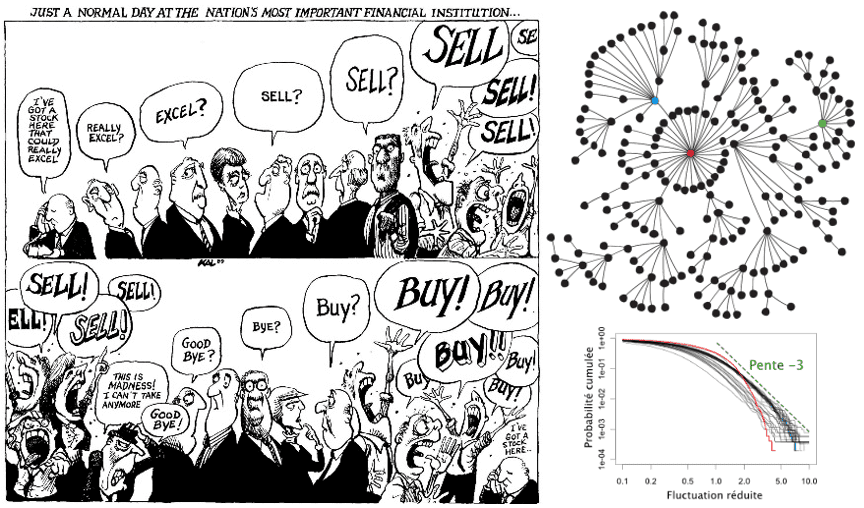
Along my readings about the analysis and modelling of the pandemy, I met several other concepts and interesting phenomenon, like i) the paradox of Simpson (nothing to do with Homer) in which global statistics give a wrong interpretation of the (detailed) reality (I strongly recommend to each of you to make a search on this paradox and read a few articles, rather at least one), and ii) the scale free networks in which the observed propagation does not follow at all a Gaussian nor a Poisson distribution, but where the amount of contacts of node can be extreme with a probability which is much higher than the one forecasted by a Gaussian or Poisson law.

For this kind of situation, the probability of extreme value is likely P(X) ≈ (1/X)^q where the exponent ‘q’ gets generally values between 2 and 3.  This means that there is no characteristic size for a population represented by this type of distribution.  The most elegant way to build a model accordingly, is to use a probability of connection to a node that is proportional to the amount of connexions the node have already got.  It has been demonstrated that this kind of networks is characterised by a P(X) ≈ (1/X)^q probability density, with ‘q’ equal to 3.

Analysis of extreme values of wins and losses on the stock exchange, after respectively a ‘buy storm’ or a ‘sell storm’ (look carefully to the cartoon on top of this article), shows that their distribution also follows this probability density, with a ‘q’ value of 3.  But the reason why remains a mystery, according to the published literature.

I will not pretend to have discovered the demonstration, but would like to give another sight on the basic pandemic distribution, i.e. the equation: (dc/dt) = k . c . (n – c), where we can see (dc/dt) as being a distribution of c, so that we have then P(C) = a . k . C . (N – C), where the factor ‘a ‘ has been introduced to ensure the sum (integral) of P(C) along the ‘c’ space (axis) is equal to 1.  P represents thus the probability to get a certain amount of people infected, when a certain amount of people is already infected.

Of course, in this space ‘C’ ∈ [0 ; N], so that the lower and upper bounds of the integral of P are respectively 0 and N.  Solving the resulting equation gives for ‘a’, the value of: (6/k.N³).  Going further, its expectancy E(C) = N/2, and its variance V(C) = N²/20 (the standard deviation being the square root of it).  It is noticeable that neither the value of E(C) nor the one of V(C) contains the factor ‘k’.  The observed average and standard deviation are independent of the transmission factor.

The value of the normalization factor ‘a’ is ≈ (1/N)^q, where ‘q’ =3.  This means, that in the ‘c’ space, the extreme values of P(C), thus the values obtained when C is near 0 and near N are in the range of 1/N³, which is precisely corresponding to the observations.  The number of soonest contaminated as well as the latest ones will be in the range of 1/N³, and so will be the value of the exchanged shares.

Now, one will say that the losses and wins on the stock exchange are values ranging from a negative minimum to a positive maximum, with their average laying around 0, while the ‘C’ space ranges from 0 to N with an average located on N/2.  No problem, let us just apply the transformation D = C – N/2, so that ‘D’ ∈ [-N/2 ; N/2].  Indeed, just a translation, to the negative direction, having an amplitude of N/2.

Applying this transformation, the ‘a’ factor remains unchanged (6/k.N³), the expectancy E(D) = 0 (what was the goal) and V(D) remains equal to V(C) (what was expected since a translation does not affect the variance), and so does (of course) the standard deviation.  The conclusions made on ‘C’ apply thus entirely, without any change, to ‘D’.

Globally said, we can conclude that the stock exchange storms, pushing the shares’ values to the sky or pressing them down to 0, are nothing else than pandemies (or buy or sell cries).  They rely subsequently on scale free networks and end up with values showing probabilities in the range of 1/value³.

The same apply to new fashion trends, which are depending on influencers who are nothing else than ‘nodes’ connected to (potential) buyer or follower ‘nodes’.  The propagation of the trend is thus also a pandemy, the contamination being achieved through selected ‘nodes’ having a lot of contacts.