The Belgian gas distribution is managed by DGO’s which measure the gas flow (in & out) at aggregated reception station (ARS) on one hand and at the entry of the customer’s premises (consumption).

The regulation defines several roles involved in gas distribution as:

• the Balance Responsible Party (BRP or Shipper), which is in charge of balancing, on an hourly basis, the demand (of the customers) and the injection (from wholesale markets/hubs) since there is no gas production in Belgium (or so few, from small scale methanisors, that they are not considered here)
• the Balance Supplier (rather the supplier in common terms), which has the (signed) contract with its customers, sources their consumption through the BRP and invoices its customers for their consumption
• the DGO’s, which achieves the distribution of the gas from the high pressure federal gas net to the low pressure customers (grid end user)
• the TSO, which manages its high pressure net (around 60 bar), consisting in hubs, connections to the high pressure net of surrounding countries TSO’s and connection to the DGO’s net

The TSO also performs the metering of the offtakes (and injections) from (into) its high pressure network, to define the infeed (total net entry, which is equal to the total net output plus the linepack which we will not consider here).

The metering on the network is performed using finely calibrated (and controlled) automated equipment, at hourly basis.  At the customers’ side, only a few are measured via automated equipment (Automatic Meter Reading: AMR), thus on hourly basis, the vast majority is measured on a (quasi) yearly basis (via index difference between 2 yearly consecutive readings; the Yearly Meter Reading: YMR) and a small part is also measured on a (quasi) monthly basis (via index difference between 2 consecutive readings achieved over roughly 25 to 35 days; the Monthly Meter Reading: MMR).

Of course, the duration between 2 readings for a YMR fluctuates around 365 days (typically 330 till 390 days), with exceptions in case of an earlier leaving, moving (in/out) of the customer.

But the Belgian allocation process runs on a monthly (calendar) basis.  The infeed is measured on an hourly basis, and the AMR at customer side too.  The remaining (YMR’s and MMR’s), which represents the major part of the total (power station offtake excluded) can only be estimated (on a monthly calendar basis).

This estimation is made using the most recent readings, stretched (up or down) to the a value representing a standard year or month (the so called Estimated Annual Volume: EAV, and Estimated Monthly Volume: EMV), which is in turn corrected to take the climate effect into account (the consumption in a month which is colder than a standard month, would be higher and conversely would be lower in a warmer month).  After this correction, the sum over the whole market still differs from the infeed minus the (the sum over the whole market of the) AMR’s, because the temperature dependence is the result of statistical model (a correlation).

Remark: to be complete, the EAV and EMV are first distributed over the hours of the month, using (3 predefined synthetic load profile curves: SLP’s, which are standard).  These curves are also the result of statistical analysis of the customers’ consumption.  But getting in this level of detail will only complicate the subject without added value.  If suitable, we can come back on this in a later paper. 

A correlation is characterized by its parameters and its quality, among them the Residu Factor (RF), through the well-known r², which is the ratio of the not explicated part of the dependence on the total dependence.

If the correlation is not biased, i.e. if the not explicated part of the correlation does not hide a variable (or a set of variables) having a measurable net effect on the analyzed dependence, then it must be normally distributed around 1 (exactly 1).

In a liberalized world there are several suppliers and BRP (private companies), while the DGO’s and TSO are monopolies.  Thus only the DGO’s and TSO dispose of data about the whole market.  Fortunately, the RF is the same for each market participant since it is no more than a stretch factor to align the bottom up sum of the distributed EAV’s and EMV’s on the infeed minus AMR’s.

Note: there is of course no RF on the AMR  since this kind of metering is achieved at the finest granularity available and does not involve an SLP nor EAV’s nor EMV’s, there are exactly known (at the measuring accuracy level).

Before starting the RF analysis, there is a last point to address, the aggregated reception station (ARS).  The gas injected into the TSO network is distributed to the end users (customers) through ARS’s.  We can figure out an ARS as a (very large) vessel in which gas is fed from the TSO network and out of which the gas is distributed to the customers through a myriad of pipes.  Of course this is an image, not the reality.  Furthermore some ARS’s are connected to other ones, not all of them.

Remark: in Belgium there exist 2 quality of distributed gas, the L-cal gas (with lower GCV, around 10kWh/Nm³) and the H-cal gas (with higher GCV, around 11kWh/Nm³).  The TSO network is also equipped with a transformer, enabling the transformation of one type into the other one (by enriching or diluting the gas in methane).  Of course the L-cal ARS’s are not (directly) connected to H-cal ARS’s, except through the transformer for the ones connected to the transformer.

The RF is calculated for each ARS, at hourly level (granularity of AMR).  Since the allocation is a (calendar) monthly process, the hourly rf (in small letters to differentiate from the RF) is commonly aggregated into a monthly value by ARS (the RF).

In Belgium there are ca. 100 ARS on the distribution network.  The allocated volume is very different from ARS to ARS and from month to month, it can go from 1 to several 100’s in relative units, while a possible volume discrepancy has a bottom value and thus affects relatively more an ARS with smaller allocated volume.  Accordingly, the RF analysis per ARS and month must be weighted by the allocated volume on this ARS and month.

With all this information, the purpose of this study is to verify whether the hypothesis of a RF normally distributed around 1 (exactly 1) can be accepted or must be rejected, at aggregated Belgian monthly level.

Remark: since the hypothesis should already be valid at ARS hourly level, the aggregation across the ARS’s and over the months should enforce the acceptation.  In other words a rejection at aggregation level (ARS’s and months) will surely lead to a rejection at ARS and at hour level, while an acceptation will not automatically lead to the acceptation at ARS and at hour level. 

Since we have used 2 aggregation parameters (ARS and month), we can challenge the hypothesis along these 2 axis too.

For our analysis, the actual µ and s are not known but estimated, so that to challenge the hypothesis we have to calculate their estimation and to use the Student distribution applied on these estimated statistics.

The test we perform has the following characterisitics:

bilateral test, hypothesis to test	H0 :  RF = 1
alternative hypothesis	H1 :   RF≠ 1
value of T under H1 (T = RF – 1)	|T| ≠ 0
significance level a	P (|T| > Tcrit) = a

 

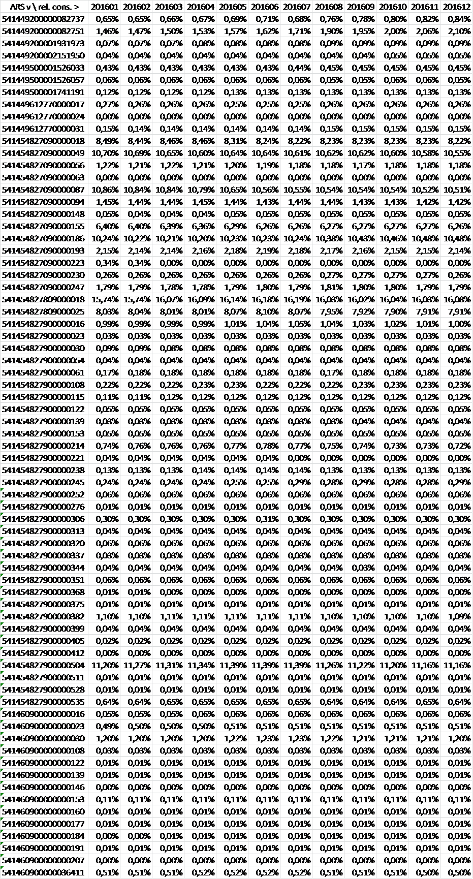
The table below figures out the RF along the months of 2016 and across the ARS’s.

For the weighting we used the SLP S41 (consumption distribution over a standard year):

and the distribution of the consumption per month across the ARS’s:

Leading to the following statistical results:

	Mean (weighted)	Standard deviation (weighted)
aggregation over the months, by ARS	0,991	0,011
aggregation across the ARS’s, by month	0,987	0,022

 

Setting the p‑critic for the ‘a’ risk on 5% (bilateral 2,5% on each side, thus t₀₂₅) leads to the conclusion that the hypothesis of RF = 1 may not be rejected.

Indeed, the confidence interval for RF is:

• aggregation over the months, by ARS: RF lays in [0,969 ; 1,013]
• aggregation across the ARS’s, by month: RF lays in [0,938 ; 1,036]

We notice that the confidence interval, calculated by ARS over the months or by month across the ARS’s, always includes 1.

Of course, as finest the p-critic as lowest the occurrence of the rejection of the hypothesis, this is inherent to the ‘a’ kind of risk (if you only convict when you have 100% certitude, the occurrence of a sentence is nearly zero).

So we will also evaluate the ‘b’ risk, i.e. the risk to accept the hypothesis while we shouldn’t which is equal to rejecting the alternative hypothesis while it is true.  The power of the test is the complementary of this risk, thus the probability to accept the alternative hypothesis while it is true.

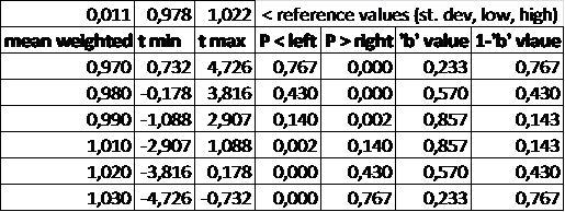
For the aggregation over the months, by ARS we have (centering the confidence interval on 1):

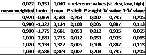
For the aggregation across the ARS’s, by month we have (centering the confidence interval on 1):

The ‘b’ risk is much lower when we analyse the RFaggregated over the months, by ARS than aggregated across the ARS’s, by month.  This means that the disparity between the ARS’s higher is than the disparity over the month, what was already revealed by the standard deviation which is twice higher.  Nevertheless, we have to temper this statement by the fact that there are only 12 months taken into account (while there are 67 ARS’s).

Extending the analysis over a longer period should lead to a reduction of the standard deviation of the aggregation across the ARS’s, by month, but to do that the ARS’s (physical) structure should also remain unchanged over analyzed period.  Unfortunately, the ARS’s structure undergoes changes over a period of 12 months (some ARS’s disappear or appear or are merged).

A power value of 0,767 is high enough to exclude differences higher than 0,03 around an RF of 1 (exactly 1).  However the power value for the aggregation across the ARS’s, by month is poor (0,205 for 0,970/1,030) which means that some ARS’s can have a different pattern.

The conclusion is that he RF for the whole market, calculated by month and analyzed over the whole year 2016 is not statistically different than a value of 1 +/- 3%, but some ARS’s can deviate substantially from this value.

This analysis concerns the whole market (aggregated) and would probably give different conclusions if applied to (very) smaller part of it, i.e. on the portfolio of a small player (BRP or supplier).

We should perhaps better draw a histogram of the RF by ARS, with the allocated volume as count (after categorization), and apply a Bayes likelihood calculation to get a finer certitude.  This could be achieved in another paper.  For the time being, we can conclude that, at whole market level, the model applied (SLP & KCF driven) is unbiased and also not distort with a structured/systematic error/dependence or hidden factor, but we can’t exclude that it is not the case at ARS level.